


Armory Sponsor


[ARCHIVED THREAD] - Reloading, Statistics and You (Page 1 of 2)
Posted: 12/28/2013 6:35:47 PM EDT
|
So I meant to do this a while back with my post 3006, but never got around to actually filling the thread out with any interesting information. I'm working on some stats tutorials for my students, so I thought this might be a nice place and time to discuss some statistical concepts, as well as put some basic instructions in for doing your own, statistically sound testing on your reloads. Questions/suggestions are most welcome. For the tl;dr crowd, there is an Excel sheet at the bottom of this post that gives some walkthrough examples.
%% --- Questions To Explore --- %% 1.) Does neck sizing vs. full-length sizing significantly affect group size? 2.) Which variable has the strongest effect on group size of these: jump to the lands, powder charge over a small range, primer type, case length? 3.) Does neck turning affect accuracy? 4.) How much does annealing brass affect accuracy? 5.) What effect does crimp have on accuracy when using bullets without a cannelure? A statistically insignificant improvement across a range of powder charges 6.) How much does neck sizing vs. full-length sizing affect brass life? 7.) Does crimping affect variation in muzzle velocity? No. Pg. 2. 8.) How often should annealing be done to improve brass life? 9.) What is the relationship between shoulder setback, brass growth and case wall thickness at the mouth? %% -----------------------------------------------------------------------------------------------------%% Instructions for Setting Up a Basic Experiment If you do nothing else, at least read and follow these instructions. Step 1: Identify the outcome or response you want to understand. For question 1.) above, we want to understand the effect on group size. Thus, we need to be able to repeatably measure group size, and that is the characteristic we're focused on. Step 2: Identify the input variable(s) of interest. It is easiest to test the effect of single variables at a time, but we can do multiple variables with careful planning (see Design of Experiments - not yet written). For question 1.) above, we want to test neck sizing vs. full-length sizing, so we have two treatments of interest. Step 3: Identify the levels of input variable you want to explore. For question 1.) above, we have two effective levels, 0 and 1 (neck sized and full length sized). This does not have to be numerical. Step 4: Identify the testing method to use. The easiest way to do this is simply ask the question in this thread as to what statistical test to use, go to that tab on the excel sheet linked at the bottom of this post, and follow the instructions, or simply find a question that is similar in nature, and do what they did. Step 5: Identify uncontrollable variables, and account for them. For question 1.) above, we'll be shooting for groups, which includes all sorts of variability, most of which comes from the human behind the rifle. You can either shoot some control groups with the study, or use several shooters through a multiple variable experiment, or simply shoot a lot of replicates, in this case. Step 6: RANDOMIZE the order in which you conduct your trials Step 7: Run the experiment. Make sure to use at bare minimum, 3 replicates (trials) for each level of each input variable. The more variation you expect, the more replicates you should run. In the case of question 1.) above, you're shooting for groups - I would shoot 5 groups of 5 shots each for each input level at a minimum (total 50 shots). Step 8: Analyze your results using the methods explained here Step 9: Believe what the data is telling you. A lot of times, data tells us things that we don't want to believe, or that fly in the face of common, non-data-based thought. Be sure to be precise about what you're saying (i.e.: if you test question 1 in single load a .30-06 bolt gun, your results are restricted to that gun and load. If you run your test in various bolt guns with various loads, then your results could be applied to bolt guns in general. If you run your test in bolt guns and autoloaders with various loads, then they are pretty general, but then you're running a MAJOR experiment - get the picture?) If you do that, you'll be conducting experiments using much better methodology than what is typical. Your results will serve you and our community much better, since they will be much more robust. If you're looking for that perfect precision load, or just trying to figure out whether reloading step X is worth your time, this is how to avoid wasting your time with an experimental approach that won't actually give you accurate results. Hypothesis Testing Example question: Is dataset A different from dataset B? This question has a lot more application than it might at first appear - this is the statistical question we would ask to answer an otherwise seemingly unrelated practical question, such as 'Does crimping reduce dispersion of muzzle velocity?', or 'Does primer type affect accuracy?' For the first question, for example, the outcome we want is to know whether or not crimping our rounds will give us an appreciable reduction in the spread (standard deviation) of muzzle velocity. To conduct this test, we would take a set of data with a crimp, and another set of data for an identical load without a crimp, and compare the two...but how? This technique is generally referred to as hypothesis testing. For most simple hypothesis testing, we develop two datasets with a single, distinguishing difference (in this case, the use or absence of a crimp). It is important to control the other variables involved, such that we can be sure the variation is resulting from what we're interested in - more on that later. We will then use what is called a test statistic to determine whether our datasets are significantly different or not. %% --- Brief, Important Aside --- %% Usually, we'll be measuring data that is somewhat random - if you measure the muzzle velocity of 5 shots, you will get random values, dancing around some mean value. If you were to fire another 5 shots from the same batch of rounds, those muzzle velocities would be different. This means that we have to characterize the difference between one dataset and another using probability, because we cannot mathematically determine for sure whether one is different from another - all we can say is "with a ___% level of confidence, this dataset is different from another one". To accomplish this, we will use certain characteristics of each dataset (mean, standard deviation, variance, pooled variance, etc.) to get an accurate picture of whether the differences between the two datasets is statistically significant. %% ------------------------------------%% So, let's say we fire 10 shots each, crimped and uncrimped. If we want to determine whether the dispersion is different, then we need to use a test statistic that compares standard deviations (in this case, we'll use variances, which is just the square of the standard deviation). We will take the variance of the first dataset, and compare it to the variance of the second dataset to determine whether there's an appreciable difference. We know that for a normally distributed dataset, if we take random samples (in this case, 10 shots), the standard deviation will vary from one sample to the next, with its own probability distribution. If we want to compare two sample variances, we would use an F-test - we would compare the relative values for the two variances to a table of standard values based on the number of trials in each sample, and the level of confidence we want in our result. If they are further apart than the table specifies (too small or too big), we rule in favor of the claim that crimping affects the dispersion of muzzle velocities. Other question types and their associated tests are listed below. Example Question: Does crimping affect variation of muzzle velocity? Statistical Question: Is there a difference between the variance of a dataset of uncrimped rounds and that of a dataset of crimped rounds? Null Hypothesis: Variance of uncrimped rounds = variance of crimped rounds Test: Inference on the variances of two normal distributions, variances unknown - we don't know the actual population variance (unless you've measured the muzzle velocity of literally hundreds of rounds with this exact load), just the sample variance. Test Statistic: F = stdev(uncrimped)2 / stdev(crimped)2 - if our calculated F is greater than the maximum indicated or less than the minimum indicated, then there is a statistically significant difference between the two variances. Example Question: Does crimping reduce variation of muzzle velocity? Statistical Question: Is the variance of a dataset of uncrimped rounds larger than that of a dataset of crimped rounds? Null Hypothesis: Variance of uncrimped rounds = variance of crimped rounds Test: Inference on the variances of two normal distributions, variances unknown - we don't know the actual population variance (unless you've measured the muzzle velocity of literally hundreds of rounds with this exact load), just the sample variance. Test Statistic: F = stdev(uncrimped)2 / stdev(crimped)2 - if our calculated F is larger than the maximum F indicated in the tables, then there is significant evidence to show that the variance of the uncrimped muzzle velocities is greater than that of the crimped muzzle velocities. Example Question: Does crimping affect muzzle velocity? Statistical Question: Is there a difference between the mean of a dataset of uncrimped rounds and a dataset of crimped rounds? Null Hypothesis: Mean of uncrimped rounds = mean of crimped rounds Test: Inference on the difference in means of two normal distributions, variances unknown - we don't know the actual population variance (unless you've measured the muzzle velocity of literally hundreds of rounds with this exact load), just the sample variance. Test Statistic: T = something awful...I'll make a graphic here or something. From there, we can determine the probability that the two values are as different as they are - if the probability is low (<5%, generally), then we can say that there is evidence to show a statistically significant difference between the muzzle velocity dispersion of crimped and uncrimped rounds. If the probability is high, then the experiment has failed to show a statistically significant difference, and the data is essentially saying that at those load conditions, there is no probable difference between the data that was measured and what would have come out in the random variation, probabilistically speaking. ----------------------------------------------------------------------------------------------------- F-Test: Comparison of Variance Let's do an example. Still asking the original question (Does crimping reduce variation of muzzle velocity?), say we take ten shots each, uncrimped and crimped, and get the following muzzle velocities [fps]:
The mean, standard deviation and variance for the two datasets, respectively, are Uncrimped: 2421 fps, 70.97 fps, 5037 fps, Crimped: 2420.5 fps, 55.50 fps, 3080 fps. We want to know if crimping reduces the dispersion (variation) of muzzle velocity. We can see that the standard deviation of the crimped velocities is 22% smaller than the uncrimped velocities, but how significant is that difference based on the data we took? If we took another pair of datasets, how certain could we be that the crimped data would come out better? This is where our test statistic comes into play - it will tell us mathematically how significant this result is. To compare these two, we will use a single-tailed F-test, as indicated above. The F-value based on our two variances in this case is 5037/3080, or 1.635. In this case, we have 9 degrees of freedom for both the numerator and denominator (the number of shots in each sample minus one), which dictates our acceptable F-values. Excel has a built-in function for this, called fdist. It works thusly: =FDIST(1.635,9,9), or =FDIST(F-value we calculated, number of shots in uncrimped sample minus one, number of shots in crimped sample minus one). This returns a value of 0.2376 - this is the level of significance in the result. Essentially, this means that we can only be 76% confident that crimped rounds have a smaller variance than uncrimped rounds. Thus, contrary to what our gut instincts tell us based on a rudimentary look at the data, there is no statistical evidence from this test to show that crimping results in less variation of muzzle velocity at a 95% level of confidence (the usual standard for such tests). Now, let's say we would like to look at the same data in a different way - let's ask the question 'Does crimping affect muzzle velocity?' This question implies that we are looking for a shift in the mean value due to crimping (i.e.: does a crimp reduce or increase the average muzzle velocity?). When looking for differences in mean values, we usually use what's called a t-test. We will characterize the two samples in terms of their averages and standard deviations, and determine the probability that they could come from the same dataset (reflecting no change due to the crimp). If the probability is lower than the confidence level we wish to see (usually 95%), then we reject the notion that they are not different (the null hypothesis). We can do this easily in Excel, either using the worksheet I have uploaded (go to the tab labeled 'Difference in Means'), or using Excel's built-in data analysis tool. If you wish to use the built-in tools, you will first need to enable them in Excel: Go to File -> Options -> Add-Ins -> Manage Excel Add-Ins -> Go, select Analysis Toolpak and click 'OK'. I'll provide instructions for use below. T-Test: Comparison of Average Values Let's look at the data again. We will use the same characteristics from the previous example (sample mean and sample standard deviation), and use a new test to determine the answer to our new question. First, we need to calculate the degrees of freedom of our data - usually, this is simply determined by the number of data points in each set minus one, but for this particular type of t-test, it is not so straightforward. If you want to see the equation, it is embedded in the Excel sheet linked below, I won't bother with it here. Essentially, the more data you have, the less of a difference you need to show between the two means in order for the result to be statistically significant. You get a higher effective number of degrees of freedom from taking more points, or having your points be close to each other, while you get a lower effective number from having fewer data points or more highly variable data. Generally, having a number of degrees of freedom higher than about 13 has diminishing returns. In the Excel sheet, we can enter the data in the rows provided (you need to manually enter the number of data points as well): 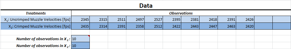
The sheet will automatically update the calculated values as your data is entered: 
The first four lines are characteristics we already calculated, so we won't discuss them. This test is showing 17 degrees of freedom, so we can expect that more data points would not change our result. Our calculated test statistic T0 is 0.00351, which is pretty low - this is essentially saying that there is about 0.3% of a pooled standard deviation between one mean and the other. Remember that for a normal distribution (comparable to a t-distribution for a high number of degrees of freedom), if we want to see a 95% probability that a point is outside this distribution, we need to go roughly 2 standard deviations away from the mean in either direction. Because we have a finite number of data points for our t-distribution, we have to show a slightly higher change, 2.11. Since we are WAY below this criterion, our p-value is very high. The p-value is the probability of obtaining the value we got for our test statistic of the null hypothesis (the notion that there is no difference between the two samples) is true. In this case, it is essentially guaranteed (99.7%) to be true. You can conduct this test easily with Excel's Data Analysis tool as well. Go to the data tab, and click the 'Data Analysis' button, usually on the right end of the ribbon. The tool we're interested in here is 't-test: Two Sample Assuming Unequal Variances'. When using this tool, simply enter your data into a blank spreadsheet the way you normally would: 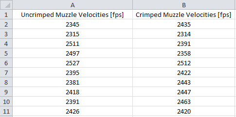
Note: it is useful to use labels on your columns, as the tool will detect this and name your data later. When you run the tool, it will present you with this dialog box: 
Click the button next to 'Variable 1 Range', and select your data, including the data label. Do the same for Variable 2. We are trying to determine whether there is any difference at all, so the hypothesized mean difference is 0. Be sure to check the Labels box to tell the program your selection includes data labels. Alpha is the level of significance we're interested in - 95% confidence in our result indicates a 5% level of significance, which is the default. Click OK, and it will create a new worksheet that looks like this: 
We see the same numbers we did in my custom worksheet, but everything is automatically calculated based on your dataset. We can use the same Data Analysis add-in to do the F-test we did originally, to determine whether our data reflects any improvement in muzzle velocity variance. Using the same data we just entered:
Go to the Data Analysis tool, but select 'F-test Two Sample for Variances'. This will present essentially the exact same dialog box as the t-test: 
Run the tool in the same fashion as before, and you will get the following results: 
Again, our P-value is 0.2376, still way too high for the significance we're looking for (<0.05). ----------------------------------------------------------------------------------------------------- Excel Practice Worksheet Here is an Excel worksheet I will be updating as time goes by (the link will change with each update) - it currently has tabs for a t-test and f-test that walks you through selecting the correct test for your question and entering your data, and it automatically calculates results for you. UPDATED 1/12/2014 Post examples of simple questions/examples you would like to see, and I'll see if I can include them in the sheet. |
|
So how do we look at changes in the behavior of data for more than two samples?
Example: in this thread, there was a discussion of IMR 4007SSC charge weight and muzzle velocity for a 308, where the author was having trouble understanding the behavior of his loads. He chronographed 5 shots each at various levels of powder charge in order to look for the charge that gave him the best muzzle velocity behavior. Here are his measurements: 44.5 2277 2403 2271 2159 2328
For starters, we know that the finite number of data points we can take cannot accurately represent the population characteristics - they are estimators (i.e.: the sample mean is a good guess for the population mean, but we will get sample means that are normally distributed about the actual mean) of the population variables. We can quantify the uncertainty in our estimate of the population mean using the following formula: 
Let's take the 44.5 grain charge weight sample - the sample mean is 2288 fps, and the sample standard deviation is 89.27 fps. As we've said before, we know if we take another sample with the exact same characteristics, we'll get different sample mean. The values we'll get are distributed according to a t-distribution with nu (the Greek letter that looks like a v) degrees of freedom equal to the number of points in the sample minus one (in this case, 4). We can estimate bounds on what value we will get 95% of the time using the above equation - the actual population mean is somewhere between 2288 fps ± 2.776*89.27 fps / sqrt(5), or somewhere between 2177 fps and 2398 fps. For reference, we can get a better estimate by taking more points in our sample (increasing N and nu, which will also slightly decrease t). If we do the same thing with the next charge weight, we get bounds of 2314 and 2564 fps, which overlap with those of the first sample - this means that there is the possibility that the actual mean value could be the same between the two groups. Boxplots Let's visualize this with a boxplot (I'll add instructions on how to do this later): 
Here's what we're looking at: the 'whiskers' on each box indicate 5% and 95% bounds on the population mean value based on the sample, respectively. The x's show the minimum and maximum actual measurements. The edges of the box represent the 25% and 75% bounds, and the little box inside each bigger box represents the sample mean. This is a valuable tool for visualizing what is happening as we vary one input variable (charge weight) - we see that there is an increase in mean value, but that the variability on the low end of the charge weight scale is so high that it makes it difficult to appreciably differentiate between the samples. If we were to repeat this test, we could greatly improve the results by taking more samples on the low end, while more samples towards the high end of the charge scale will likely not give any additional accuracy. ANalysis Of VAriance (ANOVA) We have a way to mathematically determine whether any one of these groups stick out, called an Analysis of Variance, or ANOVA. First, let's go through some terminology - we will be dealing with factors, treatments and replicates. A factor is a variable that affects the outcome, or response: in our current example, a factor would be charge weight, which affects the outcome (response), muzzle velocity. Identifying the factors in an experiment comes out of an understanding of the concept you're working with, and experience - for example, we know that outside temperature might play a part, since some powders are temperature sensitive. Perhaps primers affect it as well, and perhaps bullet seating depth - these could all be factors in the experiment. For now, let's just talk about one factor. We'll get to multiple factors later. A treatment is a specific level of a factor. In our current example, we have 5 treatments of the charge weight factor. In general, a single-factor ANOVA is looking for differences between the treatments, just as we did in our boxplot. A replicate is an observation of a given treatment - running our experiment once for each treatment level won't give us any information. In the current example, 5 replicates were taken at each treatment level (5 shots at each level of charge weight). The number of experimental trials is the number of replicates times the number of treatments. In general, 3 replicates is an absolute, bare minimum. 5 is better, and 10 is probably more than is necessary, depending on the experiment you're running. Now, before we go further, say we run this experimental example - take 5 shots at the lowest charge weight, then 5 shots at the next charge weight, etc., etc. - what is wrong with this? Well, your barrel might heat up or get fouled, your shoulder might get tired, etc. - the precise setup of the experiment will change over time. In fact, there are a number of things we may not be able to predict as changing through the course of the experiment, so we have to randomize the order in which we conduct the experiment. By randomizing order, we effectively mitigate the effect of so-called nuisance variables on our results - they should come out as homogeneous noise, which ANOVA can mathematically sort through. A good way to do this is using Excel: first, create two columns labeling each treatment/replicate pair you plan to run. In a third column, enter =RAND() and hit enter. Drag this cell's lower right hand corner down to fill all the cells where you have treatment/replicate pairs, like so: 
Now, select all three columns, click the Data ribbon, then click on Sort. It will bring up the following dialog: 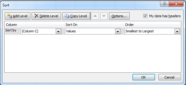
We want to sort the rows based on the random column's data - this randomizes the order of the treatment/replicate pairs for your experiment. Here is a randomized set: 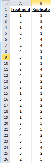
Note: the way Excel does random numbers, every time you do an Excel operation, it updates those cells with new random numbers - thus, once you've done a random sort, the rand() column will not appear to be in order, as it has been randomized again after the sort operation. You only need to do the sort once. OK, so now that we're randomizing our trials, back to our original question. The author of the thread wanted/wants to know why he's getting a dip in his muzzle velocities as he increases the powder charge. My question is whether he actually is getting a dip, i.e.: are the muzzle velocities in the group where he's getting the dip appreciably different than the levels around it? We have selected a range of treatments we're interested in (in this case, 5 levels of powder charge). We're going to replicate each treatment 5 times, and see if any of the groups stick out from the others significantly - this is precisely what ANOVA does. A caveat - in this case, the question we're looking at is a bit of a weird application for ANOVA, since we generally know that increasing powder charge increases muzzle velocity. We can glean some extra information from some post-analysis techniques, which we'll go over. Just understand for the moment that this example is just to introduce the tool. I'll post some other questions that ANOVA is more directly useful for. So here's how ANOVA works: we're going to look at the variation within the treatments themselves (essentially a grouped t-test), and compare that to the variation of the entire dataset as a whole. If the difference is significant, we know that at least one treatment is statistically different from at least one other treatment. That is ALL that ANOVA on its own can tell us - its power is limited, but important; especially for statistical phenomena we don't fully understand (there's plenty of this in reloading), determining whether changing a certain variable even causes a change in the response (the output variable we want to affect) is the first step towards figuring out how to control that response. Once we've done the ANOVA, we can do a number of things to determine which treatments caused the change, and what change was caused. -- Theory Behind ANOVA --- Here is a formal definition of the hypothesis we are testing: H0: T1 = T2 = T3 = T4 = T5 = 0, where T is the variation of each treatment from the overall mean. In other words, the null hypothesis is that the different treatments do not cause any variation from the mean. If any treatment is significantly different, we reject the null: H1: T != 0 for at least one value of T. First, let's take our dataset, and look at the mean value of each treatment level with respect to the mean value of the dataset as a whole. We can use Excel to find the average of each set of replicates discretely, then we'll subtract the overall mean value. If you see my explanation of variance to popnfresh below, that's essentially what we're going to do here: take the variation of each treatment average from the overall average, square them (such that negatives don't cancel positives), add them up, and multiply by the number of readings. This is called the Sum of Squares of the Treatments, labeled SStreatments, and represents the variation of each dataset from the total mean value. Again, what we are interested in is whether the variation of any of the treatments from the overall mean is significantly more than the random variation from the mean in each treatment (kind of a signal-to-noise ratio, if you will), which we will refer to as the error term. Those two sources of variation account for the overall dataset variation from the mean, so we can simply subtract to find it. Here's how: 1.) We have already found the Sum of Squares of the treatments (SStreatments) by squaring the difference between each treatment mean and the overall mean, then summing them and multiplying by the number of treatments: 
2.) We can find the total Sum of Squares by summing the square of each data value, then subtracting the square of the sums divided by the total number of values (yes, this is difficult to express in forum format, I apologize - it's built into the Excel practice sheet, so you can see what I mean for yourself): 
3.) We can find the Sum of Squares of the error by subtracting the value for the treatments from the total value. We then account for the number of data points figuring into each sum - the treatments value has 4 degrees of freedom (number of treatments minus one), while the error value has 20 (number of treatments times the number of replicates minus one). This gives us the Mean Squares value (MS) for each - we then use an F-test (described earlier) to compare the variation among the treatments (MStreatments) to the variation inside the treatments (MSerror). Here are the results: 
We see that the variation between the treatments is MUCH higher than the variation inside them, indicating that there is a significant difference in one of the treatments. This is reflected in our p-value of 0.016 - there is only a 0.016% probability that the null hypothesis is true (that changing the powder charge doesn't change muzzle velocity in this range). This seems kind of dumb (we know that muzzle velocity will change with powder charge, DUH!), but it can be applied to all sorts of things that are less intuitive - does crimp affect muzzle velocity? We could try three levels of crimp (three treatments), and see whether they produce appreciably different results. -- /Theory (back to the practical discussion!) --- There is an Excel tool to automatically execute an ANOVA - it is very easy to use, you just have to know how to use it. Two steps: Step 1.) Enter your reordered data (you DID conduct a RANDOMIZED test, didn't you??) into the spreadsheet. I like to do mine in rows, but you can do it in columns - you just have to tell Excel which you chose. 
Step 2.) Go to the Data tab, then click the Data Analysis button (if it isn't there, I explain how to make it appear towards the end of the first post). Select ANOVA: Single Factor, and click OK. Select your data, tell it whether the treatments are arranged by row or column, and click OK. 
It will create a new worksheet that looks like this: 
Look immediately to the p-value. If p is less than 0.05, your data demonstrates a difference from one treatment to the next. If not, the data fails to show a significant difference from one treatment to the next. Next up: identifying which treatment is best, and chasing the optimum value (this is where it REALLY GETS POWERFUL!) Taking another break, I will continue this later. |
|
This is good stuff.
I'll have to do a re-read or two and think it over before I have any hope of contributing a decent question. ETA: Holy math class, Batman! I returned to reread the OP's original post and found additional information to attempt to digest 
I look forward to returning again when I have more time and less adult beverages. |
|
Nice presentation. I am sure that some folks don't bother to run the numbers. Sometimes, it is just not in their nature to stop and study the methods, so they either skip it or get somebody else to run it for them.
I gave up wondering who was interested and who was not a long time ago. I figure if they stick around and get into it, you stop and help. If their eyes glass over or they start trying to squirm and make jokes, I just move on. Thanks for your efforts. Lets see if you get some converts. Take a look at some of this and see if you can use or build on it. http://riflemansjournal.blogspot.com/2010/07/statistics-for-rifle-shooters.html Merry Christmas and Happy New Year |
|
Quoted:
Nice presentation. I am sure that some folks don't bother to run the numbers. Sometimes, it is just not in their nature to stop and study the methods, so they either skip it or get somebody else to run it for them. I gave up wondering who was interested and who was not a long time ago. I figure if they stick around and get into it, you stop and help. If their eyes glass over or they start trying to squirm and make jokes, I just move on. Thanks for your efforts. Lets see if you get some converts. Take a look at some of this and see if you can use or build on it. http://riflemansjournal.blogspot.com/2010/07/statistics-for-rifle-shooters.html Merry Christmas and Happy New Year Thanks! Will definitely take a look! I'm working on an interactive excel sheet at the moment, need to figure out a good way to share it on the forum. Once I come up with something, I already have a couple of experiment examples with explanations and fields where you can enter your own data. |
|
Finally something interesting and useful in a tech forum rather than the same old "which press?", "best dies?", "300blk....?" rehashed, already answered questions.
I am wondering if when analyzing groups on targets for load development, if it is a waste to do low shot count groups say 3-8, then measuring actual group sizes and making determinations off those measured sizes. Wouldn't statistics be a better tool for determining what a load will actually do? I think it would better remove shooter mistakes and atmospheric changes while still actually firing the gun the way it will be fired, unlike a Lead Sled or indoor range. I don't really care what 100% of the rounds will do, I know there will be oddballs due to my mistake or whatever, I want to know, especially during load development, what I can expect of 95% of the rounds, which seems like a more realistic usable number. I understand if I shoot group after group after group I will observe a pattern and figure out what I can expect but this is very costly and time consuming. OnTarget also shows average center to center MOA, I have started paying more attention to this number than the actual group size, I just wish there was a way to get standard deviation of the group....is there? How many shots on a target would be needed to get a good standard deviation number 10-20, 20-30? |
|
Quoted:
Finally something interesting and useful in a tech forum rather than the same old "which press?", "best dies?", "300blk....?" rehashed, already answered questions. I am wondering if when analyzing groups on targets for load development, if it is a waste to do low shot count groups say 3-8, then measuring actual group sizes and making determinations off those measured sizes. Wouldn't statistics be a better tool for determining what a load will actually do? I think it would better remove shooter mistakes and atmospheric changes while still actually firing the gun the way it will be fired, unlike a Lead Sled or indoor range. I don't really care what 100% of the rounds will do, I know there will be oddballs due to my mistake or whatever, I want to know, especially during load development, what I can expect of 95% of the rounds, which seems like a more realistic usable number. I understand if I shoot group after group after group I will observe a pattern and figure out what I can expect but this is very costly and time consuming. OnTarget also shows average center to center MOA, I have started paying more attention to this number than the actual group size, I just wish there was a way to get standard deviation of the group....is there? How many shots on a target would be needed to get a good standard deviation number 10-20, 20-30? I've actually done a short study on this, and am in progress with a more significant one. These are some good questions to introduce some basics I was going to stick in one of the reserved sections as well. Will do a couple of write-ups as soon as I can ETA: Here's the brief write-up I did on the topic initially. What I have since found is that a different probability distribution tends to rule average distance to center (i.e.: it's not a standard bell curve as I assume in that write-up). More later. |
|
Quoted:
Is variance just used to magnify differences in order to better see them? I don't understand what the point is. Quoted:
Is variance just used to magnify differences in order to better see them? I don't understand what the point is. Standard deviation is actually a child of the variance, not the other way around. Picture it this way - if I want to understand how spread out my data is, what I really want to do is characterize the distance of each point from the mean. To summarize this with one number, we could take the average distance to the mean by adding all the distances, then dividing by the number of points. This presents a problem, as points less than the mean will cancel out points greater than the mean. Thus, we square the distances before adding them and taking an average - this is the variance. This isn't as useful for a direct description, as the units are now [fps2], in the case of the above experiments, while the rest of the data is in [fps]. If we take the square root of this number, we have something in comparable units that makes a little more sense, but for the mathematical operations governing a lot of statistical distributions, we use the variance. Notably, the variance is generally written down as s2, where s is the standard deviation. Also what is Population Standard Deviation? The square root of the variance or so I have read, but what is its purpose how can I use it? The population standard deviation is the standard deviation of ALL the points. 
Because 90% of the time all we have are small samples, we don't actually know a population standard deviation. If we were to repeat the same test 1000's of times, we would have a good value for this, but as it stands, we generally have to assume that we don't know what the standard deviation will be every time. Perhaps a good way of explaining this is thus: you load up 10 rounds, and take their muzzle velocities - you get an average, extreme spread and standard deviation. Do it again, same load, same rifle, same conditions, and you will get a new, and very likely different set of numbers. If you were to repeat this test again and again and again and again and again and average your SD numbers, you would arrive at the population standard deviation. Without knowing this number, however, we have to be careful in how we model the probabilities related to the small samples we do take. Does that answer your question? |
|
Quoted:
Does that answer your question? Quoted:
Does that answer your question? I think so. So population standard deviation is a more realistic prediction of what the SD would be with much more data? Thanks for answering my questions and thanks for sharing that great writeup on statistics and shot groups, that was right on point to what I was thinking. Unfortunately I don't have the math skills to do anything more than ponder. I wish something would have gotten me interested math in junior high. I am so interested now but lack even the basics and don't have the time to take classes. I have to rely online calculators. You mentioned this: Next, we can load these shots into software (or draw them on graph paper), and get some interesting
information about them. I use a script I wrote in FreeMat, an open-source MATLAB clone, to work the same way as On Target, but with quite a bit of additional functionality. Is this something I can do myself, being mathematically ignorant? Could I find the center of the group, from that center measure out to each shot center, then put those measurements into my online SD calculator or is it more complex than that? |
|
Quoted:
I think so. So population standard deviation is a more realistic prediction of what the SD would be with much more data? Quoted:
Quoted:
Does that answer your question? I think so. So population standard deviation is a more realistic prediction of what the SD would be with much more data? It is what the SD would be with much more data, yes. Thanks for answering my questions and thanks for sharing that great writeup on statistics and shot groups, that was right on point to what I was thinking. Unfortunately I don't have the math skills to do anything more than ponder. I wish something would have gotten me interested math in junior high. I am so interested now but lack even the basics and don't have the time to take classes. I have to rely online calculators. I'm happy to walk you even through the basics if you like You mentioned this: Next, we can load these shots into software (or draw them on graph paper), and get some interesting
information about them. I use a script I wrote in FreeMat, an open-source MATLAB clone, to work the same way as On Target, but with quite a bit of additional functionality. Is this something I can do myself, being mathematically ignorant? Could I find the center of the group, from that center measure out to each shot center, then put those measurements into my online SD calculator or is it more complex than that? Not more complex than that at all - yes, you can easily do it yourself. There are a couple of different ways to do it, all doable with a pencil, calipers and Excel - nothing more sophisticated than taking averages and standard deviations. The free version of OnTarget (1.10, here) also allows you to output your data to a text file format which you can then import to Excel - it gives you the point of aim, group center, and coordinates of each shot numerically. I'll be sure to do an example of this in the near future. |
|
Quoted:
I'm happy to walk you even through the basics if you like Not more complex than that at all - yes, you can easily do it yourself. There are a couple of different ways to do it, all doable with a pencil, calipers and Excel - nothing more sophisticated than taking averages and standard deviations. The free version of OnTarget (1.10, here) also allows you to output your data to a text file format which you can then import to Excel - it gives you the point of aim, group center, and coordinates of each shot numerically. I'll be sure to do an example of this in the near future. OK, that seems to work. I opened a target I had in OnTarget,saved it as text, I don't have a clue how to put these numbers into Excel so I used my CAM/CAM software to plot the center and the shot points then dimensioned them from the center point of the group, I then took these distances and plugged them into the online SD Calculator. The mean on the calculator was the same as the average center to center distance that OnTarget showed so I must have done something right. So now I assume I would have to multiply the SD(or would I use population standard deviation) number by 2 to get the diameter then divide by 1.047 to get MOA. So what can I predict from this? The pop SD was .4875" or if I assumed correctly, .931MOA. Does that mean 68% of the shots will be within .931MOA, 95% of the shots will be within 1.862MOA and 99.7% of the shots will be within 2.973MOA? |
|
Quoted:
OK, that seems to work. I opened a target I had in OnTarget,saved it as text, I don't have a clue how to put these numbers into Excel so I used my CAM/CAM software to plot the center and the shot points then dimensioned them from the center point of the group, I then took these distances and plugged them into the online SD Calculator. The mean on the calculator was the same as the average center to center distance that OnTarget showed so I must have done something right. So now I assume I would have to multiply the SD(or would I use population standard deviation) number by 2 to get the diameter then divide by 1.047 to get MOA. So what can I predict from this? The pop SD was .4875" or if I assumed correctly, .931MOA. Does that mean 68% of the shots will be within .931MOA, 95% of the shots will be within 1.862MOA and 99.7% of the shots will be within 2.973MOA? Quoted:
Quoted:
I'm happy to walk you even through the basics if you like Not more complex than that at all - yes, you can easily do it yourself. There are a couple of different ways to do it, all doable with a pencil, calipers and Excel - nothing more sophisticated than taking averages and standard deviations. The free version of OnTarget (1.10, here) also allows you to output your data to a text file format which you can then import to Excel - it gives you the point of aim, group center, and coordinates of each shot numerically. I'll be sure to do an example of this in the near future. OK, that seems to work. I opened a target I had in OnTarget,saved it as text, I don't have a clue how to put these numbers into Excel so I used my CAM/CAM software to plot the center and the shot points then dimensioned them from the center point of the group, I then took these distances and plugged them into the online SD Calculator. The mean on the calculator was the same as the average center to center distance that OnTarget showed so I must have done something right. So now I assume I would have to multiply the SD(or would I use population standard deviation) number by 2 to get the diameter then divide by 1.047 to get MOA. So what can I predict from this? The pop SD was .4875" or if I assumed correctly, .931MOA. Does that mean 68% of the shots will be within .931MOA, 95% of the shots will be within 1.862MOA and 99.7% of the shots will be within 2.973MOA? To import the data from the text file in Excel, just go to File -> Open, then select 'All Files' in the filetype dropdown, then open the text file. The default values for the text import dialog are correct (Delimited, then Tab), so just click Next, Next, then Finish. It will give you your data in cells like this: 
The listed group center point is equal to the average x and y position values. The distance of each point from the center point is simple using the Pythagorean theorem: calculate the x and y distances from the average, then square them, add them, and take the square root. This gives you the radius, r, of each shot to the center of the group. Here's an example: 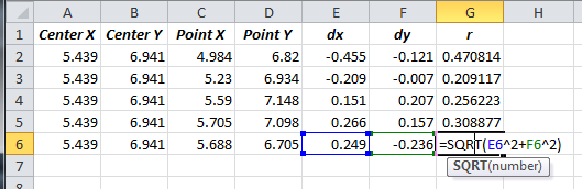
You can then use =average() and =stdev() to calculate the mean and standard deviation of your shot radius to group center, and go from there. In my case, I had a mean radius to the center of the group of 0.318" and a standard deviation in the radius to group center of 0.0997". Using a normal distribution as I did in the paper actually turns out to be an inaccurate way to model the shot placement behavior, as I found out in subsequent tests after writing that piece. We have to use a different probability distribution all together - I ran a postal match and had some precision shooters essentially give me gobs of data to work with, and I found a better (much more accurate) method for estimating shot probabilities. I'll see if I can dig up the work I did on it and finish explaining how. Let me know if you have problems getting this far. |
|
Quoted:
I don't generally do the sort of shooting that calls for the sort of analysis you're doing here, but the effort is appreciated nonetheless. This is an OUTSTANDING thread and I'm glad I found it. +1 Way more than what I need but good stuff to know and consider. Thanks for the hard work and attention to details. I'll have to read over it again... |
| Update: Fixed link with google drive upload. Let me know if it doesn't work - when you're looking at the viewer, the download button is towards the upper left of the screen (it's an arrow). Working on two-way ANOVA example related to a current thread on the effect of crimping. |
|
OK, so for an example, I'm going to run an experiment looking at the effect of primer type and crimp on muzzle velocity. Specifically, my question is:
Do primer type and crimp affect variation in muzzle velocity? For this test, I'll use two primer types - CCI 200 LR and CCI BR-2 primers. I have loaded up a bunch of 308 rounds with the following load characteristics: R-P Brass, sized to SAAMI minimum headspace (my LR-308 chamber is TIGHT), and trimmed to 2.005. Hornady 168 A-max 38.0 ±0.1 Grains IMR 8208-XBR CCI 200/CCI BR-2 primers 0.0018" neck tension COL 2.788" Crimped rounds crimped with 1/2 turn of Lee FCD, approximately 0.0008" The null hypothesis I'll be testing is: H0: Primer type and existence of a crimp do not affect muzzle velocity variation for this load. The alternative hypothesis is: H1: Either primer type, crimp, or the interaction of the two affects muzzle velocity variation for this load. 
I have loaded 40 rounds (with 5 additional sighters/control/spares), 20 with CCI 200's and 20 with CCI BR-2 primers. Half of each primer type (10 rounds of each) has had a taper crimp applied, while the other half has not. The key is to be as consistent as possible with variables that are expected to affect the outcome, and to treat those you cannot control as nuisance variables. In this case, I have only a limited amount of this consistent headstamp brass. As a result, I can't just throw out brass of a different weight, which has been supposed by many to significantly affect muzzle velocity (it has not in my tests, but whatever). So, I randomized the weight distributions throughout the loading. A good way to do this s to toss the brass in a big bag, jumble it around a bit, and load them up at random. I have noted their weight with their position in the cartridge box, which will be very useful data later - we'll essentially get a twofer with this single experiment. OK, so here's how it works - I'm going to fire the rounds at a target, with a specified period of time between shots for consistency. I will fire them one at a time in a randomized order, noting their muzzle velocities and position on target. I will put the case back in its original slot in the box so I can take post-experimental measurements later if I want. I will shoot in the middle of the day so as to try for a consistent temperature, but 8208 is supposed to be a pretty temp-stable powder. I hope to shoot this tomorrow, then I'll walk through the analysis method |
|
Very interested in the outcome of this. Was there any reason you chose to stick with the CCI primers for both tests?
I'm assuming it was just what you had on hand, but thought I'd ask. Do you think it would have been worthwhile to try a different brand of primer in your test? -ZA |
|
Quoted:
Very interested in the outcome of this. Was there any reason you chose to stick with the CCI primers for both tests? I'm assuming it was just what you had on hand, but thought I'd ask. Do you think it would have been worthwhile to try a different brand of primer in your test? -ZA Just what I had on hand. It would definitely be interesting to add different primers in the future. BTW, you have a package inbound 
|

|
question:
maybe this has been addressed, and I just missed it. however, in your questions that you are trying to answer statistically in the first post, it always mentions accuracy. am I reading it wrong? or was there an assumption made and called out? edit: nevermind, read it again and understand... comprehension isn't great with near zero sleep and early in the morning before coffee. |
|
We do it the old fashioned way. .260 Rem. with 1.5 inch groups at 1000 yds.
Understanding the physics of the cartridge/chamber/barrel , in my opinion, are far more important than the raw data one might accumulate. When you KNOW the throat erosion rate in inches along with SD`s of zero it gets easier. Sartorius scale for the win. I really don`t care about the statistics since my shooter has an MBA. I don`t have to spend time on things that I can`t control. |
|
Quoted:
We do it the old fashioned way. .260 Rem. with 1.5 inch groups at 1000 yds. Understanding the physics of the cartridge/chamber/barrel , in my opinion, are far more important than the raw data one might accumulate. When you KNOW the throat erosion rate in inches along with SD`s of zero it gets easier. Sartorius scale for the win. I really don`t care about the statistics since my shooter has an MBA. I don`t have to spend time on things that I can`t control. My focus in this thread is on presenting how to use a statistically and scientifically sound methodology for testing concepts related to reloading. If you'd like to start your own thread on your approach, I'm sure I'd find it plenty interesting |
|
Quoted:
My focus in this thread is on presenting how to use a statistically and scientifically sound methodology for testing concepts related to reloading. If you'd like to start your own thread on your approach, I'm sure I'd find it plenty interesting Quoted:
Quoted:
We do it the old fashioned way. .260 Rem. with 1.5 inch groups at 1000 yds. Understanding the physics of the cartridge/chamber/barrel , in my opinion, are far more important than the raw data one might accumulate. When you KNOW the throat erosion rate in inches along with SD`s of zero it gets easier. Sartorius scale for the win. I really don`t care about the statistics since my shooter has an MBA. I don`t have to spend time on things that I can`t control. My focus in this thread is on presenting how to use a statistically and scientifically sound methodology for testing concepts related to reloading. If you'd like to start your own thread on your approach, I'm sure I'd find it plenty interesting And what a great presentation it is! I simply don`t understand it. I have zero background in stat. Never took a single class,,,hence my confusion. lol. My son took three classes in your discipline and will surely enlighten me when I show him your thread. My comment was meant to show that empirical data sometime serves a purpose particularly for our specific endeavor. Our reloading centers around repeatability coupled with a complete understanding of how the projectile behaves along its trajectory going down range.
|
|
I just wanted to chime in and congratulate you on contributing something technical to a site devoid of this type of thing. If you need any help, I'm working on my Ph.D. in AE (I'm assuming you majored in this also, rocketman?), and one of my quals areas was systems design. Also, I'm assuming you're providing Excel examples so that other people can use them. But, for your own use, have you ever used JMP? It's nice for these sorts of things, especially for creating DoE tables. Again, great contribution.
|
|
Quoted:
I just wanted to chime in and congratulate you on contributing something technical to a site devoid of this type of thing. If you need any help, I'm working on my Ph.D. in AE (I'm assuming you majored in this also, rocketman?), and one of my quals areas was systems design. Also, I'm assuming you're providing Excel examples so that other people can use them. But, for your own use, have you ever used JMP? It's nice for these sorts of things, especially for creating DoE tables. Again, great contribution. My PhD is in ME, but my background is mostly from industry - I came back to school after about 10 years doing various jobs in machine design and manufacturing. The standard packages where I worked in industry were JMP and Minitab - they're definitely more tailored for this sort of thing, but I figured everybody here would at least have access to Excel Glad you appreicate the thread, let me know if there are ways I can improve it. I have some test materials headed to ZA from another thread, we'll post up our test results both in that thread and in here, for posterity. Hopefully, that will be enough to get people excited to ask other questions |
|
OK, so I have the results from my crimping experiment in 308. We can look at this a number of different ways - we'll start simple. For the moment, let's just look at the rounds primed with CCI 200's. Here is the load data:
R-P Brass, sized to SAAMI minimum headspace (my LR-308 chamber is TIGHT), and trimmed to 2.005. Hornady 168 A-max 38.0 ±0.1 Grains IMR 8208-XBR CCI 200 primers 0.0018" neck tension COL 2.788" Crimped rounds crimped with 1/2 turn of Lee FCD, approximately 0.0008" For this first run at the data, the null hypothesis I'll be testing is: H0: Crimp does not affect variation in muzzle velocity for this load. The alternative hypothesis is: H1: Crimping affects variation in muzzle velocity for this load. Here's how I conducted the experiment: First, I loaded the rounds, noting the weight of each case (more on this later), and arranging the loaded rounds in an ammo box, as pictured above. I set up a target at 50 yards, with a Shooting Chrony F1 Master (measurement uncertainty of ±0.5% of the reading) set up at 10 yards from the muzzle. I used the rand() function in Excel to randomize the shot order, and fired timed shots over the chrony, with 1 minute in between shots. Here is the raw data: 
We can make a boxplot straight away, for a visual check: 
We can see that the standard deviation of the uncrimped group is very slightly smaller than that of the crimped group, but they appear far too similar to know whether this result is of any significance. We also see that there is nearly no change in average muzzle velocity. To actually do the comparison, we need to calculate - here, we'll use a single-factor, two-tailed ANOVA (ANalysis Of VAriance) to analyze the data. Here are the results: 
We get a p-value of 88%. In other words, there is an 88% chance that the null hypothesis is correct. Thus, we fail to reject the null hypothesis - in other words, in this experiment, we found no significant evidence to suggest that crimping this load affects the variation in muzzle velocity. TL;DR crimping had no significant effect on muzzle velocity dispersion. BONUS: Since we measured the case weights (actually, of the whole test, both primer types), we can see whether there's a relationship between case weight and muzzle velocity. Here's the plot: 
From appearance, it's highly unlikely that there is a repeatable effect of case weight on muzzle velocity for this load. This agrees with test results I have had with .30-06 loads - sorting case weights had no measurable effect on muzzle velocity variation. Thus, I don't bother with it anymore More later |

|
Nice test RocketmanOU.
By chance, did your test include any observations on accuracy or precision? What method do you like to use for charge weights? Is that really a +/- 0.1 grain uncertainty in the charge weights or the range on a scale reading? I get about the same extreme spread on brass weights as your tests, roughly about 13 grain spread (+/- 3 sigma), but I don't get a correlation to internal case volume. Have you checked case volume at the tails? Do you weight sort bullets to check for flyers, or just accept all samples? I am often surprised by the flyers I find in terms of bullet weights. |
|
Quoted:
Nice test RocketmanOU. Thanks By chance, did your test include any observations on accuracy or precision? This test did not - the one ZA206 and I will be simultaneously running on 223 in the very near future will. What method do you like to use for charge weights? Is that really a +/- 0.1 grain uncertainty in the charge weights or the range on a scale reading? Depends on what I'm doing, and what powder I'm using. In this case, I wanted to eliminate variation in powder charge as a variable as much as possible, so I trickled the loads - the error on my scale is ±0.1 grains. In general, I have found for most rifle case volumes (223 and up, certainly 243, 308 and 30-06) that slight variations in powder charge don't much affect muzzle velocity for tuned loads. When just loading plinking rounds, I don't even think about it and leave it up to the meter. When loading precision rounds, part of my load workup is looking at the effect of powder charge variation. Usually it's small enough that going beyond normal metering has little to no benefit. When eliminating it as a variable, however, it is important to try to control it - in this case, I was using a stick powder that meters decently well, but I wanted to be sure. If I were using a ball powder, I would meter it, as the meter will likely throw more consistently than I can trickle. I get about the same extreme spread on brass weights as your tests, roughly about 13 grain spread (+/- 3 sigma), but I don't get a correlation to internal case volume. Have you checked case volume at the tails? Internal case volume does not correlate well with case weight. I have tried this several times, and the results are generally poor in terms of an observable relationship. I kept my cases in the ammo box in order, so I could add water volume data, but it would be after the cases have been blown out to the chamber walls, so it's unlikely to give good results. You may find a correlation between case volume and muzzle velocity, but I honestly doubt you will. In any case, sorting cases by weight seems awfully foolish, given the data I've collected on various loads. In my testing, I've generally seen exactly what it looks like above - no conclusive relationship between muzzle velocity and case weight, nor between muzzle velocity variation and case weight variation. In fact, in the last test I ran on .30-06, properly prepped brass with a higher variation in case weight produced not only more consistent muzzle velocities, but more accurate groups. Don't tell the benchrest guys, they'll call me a heretic and burn me at the stake. 
Do you weight sort bullets to check for flyers, or just accept all samples? I am often surprised by the flyers I find in terms of bullet weights. Depends on the bullet. Hornady A-max and Sierra Matchkings, I usually can't measure any difference. In this case, I weighed the Amax's just to see, and they were within ±0.1 grains, easily. Off-brand bullets or seconds, you can usually detect a difference. I have a batch of 168 grain bullets from Grafs IIRC that have variations up to ±4 grains |
|
Questions added to OP pursuant to Scorpius's fine thread here
He did a very interesting test regarding brass life and annealing with his Giraud annealer. I'll be combing through his data to see if we can easily draw from what he's already done, and we'll see if we can extend his study with a few easier tests. Namely, it seems from his data that annealing's effect on case life is limited until a high number of firings. There seems to be a significant effect based on these initial graphs (i.e.: annealing vs. not annealing increased maximum case life), but the median case life (12 shots) was unaffected by the annealing factor. Here are the initial graphs: 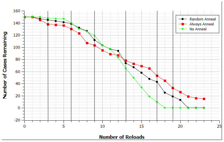
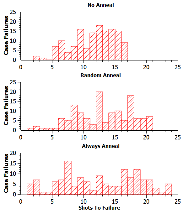
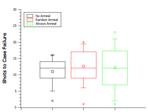
Once Scorpius sends me his raw data, I'll see what else we can discover |
[ARCHIVED THREAD] - Reloading, Statistics and You (Page 1 of 2)
Armory Sponsor